Tuesday, March 22, 2016

Convert numbers into words in Excel

How to you ask excel to convert a numerical value into a text interpretation. This is mostly handy in currency data.

Here is how:

Use the below formula and have the reference corrected.

=TEXT(A1,CHOOSE(INT(LOG10(A1)/3)+1,"#","#,","#,,","#,,,","#,,,,")) &CHOOSE(INT(LOG10(A1)/3)+1,""," Thousand"," Million"," Billion"," Trillion")

Well, I hope you have enjoyed this. Let me know if you want to know something more or have any specific question (questions.aweexcel@gmail.com)

Monday, March 21, 2016

How to filter pivot tables based on a cell value

Ever wondered how convenient would it be if all the filters of all the pivot tables changed based on a cell value.

Yes, you can do it using the below VBA code.

The steps are as follows.

1. Copy the below VBA code.

Private Sub Worksheet_Change(ByVal Target As Range)

Application.ScreenUpdating = False

Application.ScreenUpdating = False
Dim PT As PivotTable
Dim pi As PivotItem
Dim strField1 As String
Dim strField2 As String


strField1 = "School"


On Error Resume Next
Application.EnableEvents = False
Application.ScreenUpdating = False
a
If Target.Address = Range("B2").Address Then

For Each PT In PivotTables
With PT.PageFields(strField1)
For Each pi In .PivotItems
If pi.Value = Target.Value Then
.CurrentPage = Target.Value
Exit For
Else
.CurrentPage = "(All)"
End If
Next pi
End With
Next PT
End If

If Target.Address = Range("B2").Address Then

For Each PT In PivotTables
With PT.PageFields(strField2)
For Each pi In .PivotItems
If pi.Value = Target.Value Then
.CurrentPage = Target.Value
Exit For
Else
.CurrentPage = "(All)"
End If
Next pi
End With
Next PT

End If

Application.EnableEvents = True
Application.ScreenUpdating = False

End Sub

2. Right click on the excel sheet where you have your pivot tables. Now click on 'View code'


3. Now paste the code you have copied and make the following changes as applicable in your case.

  • Change the "Range(XX)" references in the code to the cell where you would input the filter value.

  • Change strField1 = "XXXXXX" to the actual field in the pivot able on which you would apply filter for.

4. Save the file as a Macro-enable excel file. Re-open the file and enter any available value for the field you want to filter for in the Range you have specified .


Done!! You have done it. :)

Well, I hope you have enjoyed this. Let me know if you want to know something more or have any specific question (questions.aweexcel@gmail.com)

How to count unique values in Pivot table

This is a very interesting problem where in many data analysts find pivot table worthless when it comes to counting distinct(or unique) occurrences of a value in a table.

The solution is as below.

Example:

Basically you want to count unique occurrences of each value from the column 'List'

1. Add an additional column next to it and input an array formula (for indexing) which would basically sort the values in a more meaningful order.


Formula at cell C3 is: 
=INDEX($B$3:$B$17,MATCH(SMALL(COUNTIF($B$3:$B$17,"<"&$B$3:$B$17),ROW(A1)),COUNTIF($B$3:$B$17,"<"&$B$3:$B$17),0))

Ctrl+Shift+Enter 
(to make it an array formula)

the above step is optional and can be skipped if concerned.

2. Now add another column 'Count' with the following formula. This countif formula would divide the total occurrences to fractions that would some up to '1'.


Formula at cell D3: 
=1/COUNTIF($C$3:$C$17,C3)

3. A pivot of the table (B2:D17) with the column 'Count' in the values field will show the unique count of each values in either 'List' or 'Array formula' column.


Well, I hope you have enjoyed this. Let me know if you want to know something more or have any specific question (questions.aweexcel@gmail.com)

Below is the link to the excel file I am talking about. 


Friday, March 18, 2016

INDEX MATCH versus VLOOKUP functions - Microsoft Excel

Most of the folks who use Excel do not know that a alternate combination of functions is available for Vlookup. In this post I would explain:

1. Drawbacks of Vlookup function
2. Best alternative for Vlookup function.
3. Usage of index and match function.

Vlookup is a function which allows users to lookup for a particular value in a column and provide the related data of that value from the subsequent columns towards right side.

1. Drawbacks of Vlookup function:

  • You cannot lookup for values towards the left of the table from where the lookup value column resides.
  • Generally Vlookup is not recommended if you are performing the lookup on a huge dataset. As this uses a lot of system's resources rendering the Excel application useless until the lookup calculation is completed.
2. Best alternative for Vlookup function.

INDEX and MATCH functions are a good alternative for Vlookup as they overcome the drawbacks mentioned earlier.

3. Usage of index and match function.

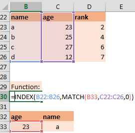
Index & Match example:

Example 1: Right hand side lookup from a table


Example 2: Left hand side lookup from a table

Hopefully you have enjoyed the tip. Let me know if you want to know something more or have any specific question (questions.aweexcel@gmail.com)

First Post! - Welcome

Welcome guys to my new blog focusing on learning aspects in Microsoft Excel.

I will try and cover wide range of topics on Excel and hopefully this blog will serve as a good resource to you.

You can send me your queries on anything related to Microsoft Excel at questions.aweexcel@gmail.com